Technical Notes

Stages of Carbon Capture Storage

CO₂ concentration in the atmosphere

Seen over a period of millions of years CO₂ has an interesting and life-giving history. Without CO₂, there would not have been the kind of life on earth we see today. The atmosphere today consists of about 78.08% nitrogen (N2), 20.95% oxygen (O₂), 0.93% argon (Ar) and 0.04% (about 400 ppm) CO₂, but it has not always been like that. The atmosphere would have contained no O₂, had it not been formed by the photosynthesis of green plants, and without that more than 21% (210,000 ppm) of atmospheric air would have been CO₂, disregarding the water content. From the day green plants arose around 700 million years ago, they began to consume CO₂, which as shown in Figure 1 was used as a building material to form glucose (C₆H₁₂O₆) and oxygen (O₂). This process is called photosynthesis. For plants, O₂ is a waste product, but the animals and humans who later populated the earth reversed the chemical reaction in Figure 1 by consuming plants and other animals. This released CO₂, which in turn could be used as building material by the plants.

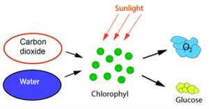
Figure 1 Photosynthesis.

Not all organisms are consumed by other organisms. Some are buried underground and over time turned into gas, oil, or coal. With each organism buried, humans and animals were giving less CO₂ back to the atmosphere than consumed. A hundred years ago, the CO₂ concentration in the atmosphere had dropped to about 280 ppm (0.028%). A drop in atmospheric CO₂ concentration from more than 210,000 ppm when green plants appeared to around 280 ppm may seem quite dramatic but given that it happened over a period of about 700 million years, the annual decrease in CO₂ concentration is only of the order of 0.3 parts per billion and has hardly been felt within a few generations. With a continued steady annual decline in CO₂ concentration, it would take about a million years for the CO₂ to be used up and all life would die out.
Throughout history, there have been fluctuations in the CO₂ concentration in the atmosphere. Measurements suggest that the CO₂ concentration during the last glacial period, about 20,000 years ago, was as low as 180 ppm. Cold water can dissolve more CO₂ than hot water. Degassing of CO₂ from seawater is therefore believed to be a major source of the increase in CO₂ concentration in the atmosphere from about 180 ppm to 280 ppm that happened from the time about 30% of the earth was covered by ice to the start of the modern industrial age about 100 years ago.

CO₂ is produced when burning methane (CH₄), other hydrocarbons, and coal. This could be seen to bring some of the CO₂ originally in the atmosphere back to the atmosphere. However, if more CO₂ is produced from respiration of living organisms and by burning fossil fuels than consumed by plants and trees, the CO₂ concentration in the atmosphere will increase as opposed to what has happened for the millions of years with a net removal of CO₂ from the atmosphere to carbon compounds buried underground. If all the carbon were taken up from the underground and burned, one must expect the CO₂ concentration to return to the 21% level it had when the first green plants appeared, in which environment no animal species would survive.

CO₂ quantities produced by combustion

The chemical reaction for burning of methane (CH₄) is:

CH₄ + 2O₂ → CO₂ + 2H₂O

Table 1 shows a typical reservoir oil composition. As is detailed in the table, burning 1 mole (=107.96 g) of oil will produce 344.18 g CO₂. The weight amount of CO₂ produced is in other words 344.18/107.96 = 3.19 times higher than the weight amount of the reservoir oil.

Table 1 Oil compositions and weight amount of CO₂ produced by burning 1 mole of oil.

At reservoir conditions, CO₂ and the oil in Table 1 will have approximately the same density. The CO₂ formed by burning 1 reservoir cubic meter of oil will thus occupy a volume of around 3 cubic meters at reservoir conditions. As sketched in Figure 2, storing CO₂ in depleted oil fields will therefore only provide space for one third of the CO₂ produced. If the CO₂ concentration in the atmosphere is not to increase, space must be found elsewhere for two thirds of the CO₂ produced.

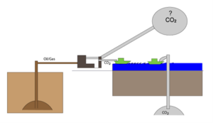
Figure 2 Illustration of the fact that depleted oil reservoirs can only hold a third of the CO₂ produced by burning oil and gas.

CO₂ capture

The oxygen (O₂) needed for the combustion of gas and oil comes from atmospheric air. Table 2 shows the compositions of atmospheric air and of a typical combustion gas.

Table 2 Composition of atmospheric air and a typical combustion gas.

Before CO₂ is disposed of, it must be separated from N₂ and other gases. This can be done using an amine absorption process as sketched in Figure 3. CO₂ is absorbed when the combustion gas contacts the amine (MEA) solution, while N₂ and other gases are discharged at the top. The absorbed CO₂ is separated from the amine solution in a heater.

The chemical reactions are:

Absorption:
MEA + CO₂ → MEACOO^– + H⁺

Bicarbonate formation:
MEACOO^– + H₂O → MEA + НСO^–₃

Desorption:
HCO^–₃ + H⁺ → CO₂ + H₂O

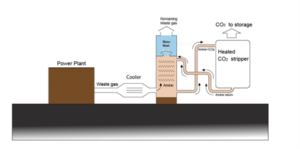
Figure 3 Amine absorption unit for separating CO₂ from other gases contained in combustion gas.

CO₂ at pipeline and storage conditions 

Figure 4 shows the phase diagram of CO₂. The CO₂ molecule is linear, which in both the liquid and the vapor state favors a high density. The linear shape is also the reason CO₂, compared to other components of approximately the same molecular weight, solidifies at a higher temperature.

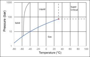
Figure 4 CO₂ phase diagram.

Ship transport of CO₂ will most often take place with CO₂ placed in insolated cryogenic tanks, where the temperature is around -46°C and the pressure high enough to ensure that the CO₂ is in liquid form, which means 8 bar or slightly higher. In a pipeline, the temperature will be determined by the ambient temperature, which will often be 4-30°C. The pressure is adjusted to ensure the density is high, without requiring an unreasonable compressor capacity. This is achieved at a pressure of 80-150 bar. Underground storage of CO₂ in depleted oil fields or in aquifers could take place at a temperature of around 75°C and a pressure of around 225 bar.

Figure 5 shows the density of CO₂ at typical shipping, pipeline and aquifer conditions. In marine transport, the CO₂ density exceeds that of pure water, while at pipeline conditions the density is slightly lower, but still high considering that it is a condensed gas component. At aquifer conditions, CO₂ is supercritical, but the density is still relatively high. 

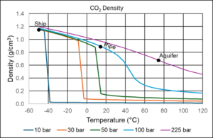
Figure 5 CO₂ density at typical shipping, pipeline, and aquifer conditions.

Pipeline transport of CO₂

In a pipeline, it is preferable to transport CO₂ as single-phase liquid, but two-phase transport may occur. If so, it will be at temperature and pressure conditions located somewhere on the vapor pressure curve in Figure 4. This is a major difference compared to gas and oil mixtures, for which the two-phase region may cover a large PT area. This does not mean that the change from gas to liquid is instantaneous in a pipeline transporting CO₂. Both gaseous and liquid CO₂ can be present over long pipe distances, possibly in the entire pipe.

When carrying out flow simulations for a pipeline transporting gas and oil, it is for each section calculated how the heat (enthalpy) exchanged with the surroundings affects the relative phase quantities, their composition, and the temperature in the pipeline. This can either be done by table look-up or by continuously calculating how the phase quantities and compositions at the current pressure change with temperature. That method cannot be used for pure CO₂. For a given pressure, the temperature remains fixed as long as two phases are present.

Figure 6 shows a Pressure-Enthalpy diagram for CO₂. If two phases exist at a temperature of 10°C, the pressure is approximately 45 bar. The liquid phase will have an enthalpy of around -260 kJ/kg and the gas phase an enthalpy of around -63 kJ/kg. The total fluid will have an enthalpy in that range and the relative amounts of gas and liquid are determined using the lever rule.

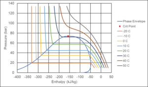
Figure 6 Pressure-Enthalpy (PH) diagram for CO₂. The enthalpy reference state is ideal gas at 0°C. 

Should a leak occur on a pipeline transporting natural gas, the leaking gas will rise into the air because the molecular weight of natural gas (18-20) is lower than that of atmospheric air (around 28.964). CO₂ has a molecular weight of 44.0 and it will take time before the leaking CO₂ mixes with the atmospheric air. In calm weather, CO₂ from a leaking CO₂ pipeline could form a kind of blanket around the leak and pose a hazard to people nearby.

Thermodynamic properties of pure and lightly polluted CO₂

Thanks to the many industrial uses of CO₂, good, validated, and easily accessible models exist for describing the properties of CO₂. The volume-corrected SRK and PR equations are the industry standard for oil and gas and can also be used for CO₂. In case more accurate CO₂ properties are needed, one may use the Span-Wagner equation [1] developed for pure CO₂, or the GERG-2008 equation [2]. The latter can handle mixtures of up to 20 specific components including CO₂.

The CO₂ to be transported and stored underground will seldom be pure CO₂. Figure 7 shows the phase diagram of CO₂ with trace amounts of nitrogen, argon, and water. It illustrates the fact that liquid water may well form in a pipeline transporting lightly polluted CO₂. This may lead to corrosion problems as dealt with later. The industry standard SRK and PR equations are also applicable to mixtures with water, but it requires modifications capable of describing that water molecules when mixed with other components do not distribute randomly but prefer other water molecules as their nearest neighbors. Such modifications of the classical cubic equations are well described in the literature [3a].

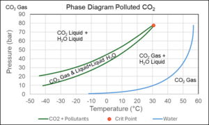
Figure 7 Phase diagram of mixture consisting of 97.7 mol% CO₂, 1.6 mol% N₂, 0.3 mol% Ar, and 0.4 mol% H₂O.

Even trace amounts of water can lead to the formation of CO₂ gas hydrate. This is a solid with properties similar to ice that can form at temperatures significantly higher than 0°C, which is the freezing point of water. Figure 8 shows a phase diagram for CO₂ with trace amounts of water. As is seen from the figure, gas hydrate formation will only occur if some CO₂ is in gaseous form, or the temperature is lower than around -13°C.

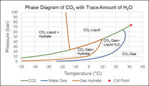
Figure 8 Phase diagram of mixture 99.9 mol% CO₂ and 0.1 mol% H₂O.

CO₂ storage in depleted oil fields

The most obvious storage sites for the CO₂ produced by burning oil and gas from petroleum reservoirs are the same reservoirs after the production by natural depletion has stopped. CO₂ gas injection into oil fields has for many years been used as an enhanced oil recovery (EOR) technique. The injected CO₂ mixes with the oil left in the depleted field and forms a zone that propagates through the field and pushes the oil forward towards the production well. It is a known and safe technique as long as the pressure in the reservoir does not exceed the original reservoir pressure. The mechanisms behind miscible gas displacement are well documented [3b]. Although this is an obvious storage option, additional storage space must be found because, as already mentioned, the CO₂ produced takes up three times the volume that the produced oil or gas leaves in the reservoir.

CO₂ storage in aquifers

The term Carbon Capture and Storage (CCS) was first used in the early 2000s. It was the time, it became clear that a new technical discipline was needed if virtually all CO₂ from combustion gases were to be captured and purified, and sufficient storage space were to be found for the purified CO₂. Brine reservoirs are present in large numbers worldwide and could be candidates to provide the additional storage capacity needed beyond that found in depleted oil fields.

The solubility of CO₂ in saltwater is much lower than in oil. As illustrated in Figure 9 an aquifer volume of around 50 m³ would be needed if the CO₂ produced by burning 1 reservoir cubic meter of oil were to dissolve in a brine aquifer [4].

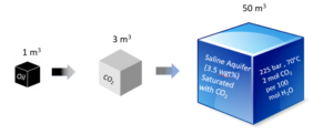
Figure 9 Volumetric development from oil at reservoir conditions to CO₂ at reservoir conditions to CO₂ dissolved in a brine aquifer.

According to the International Energy Agency, CO₂ emissions in 2023 from the combustion of fossil fuels were 37.4 billion tons. If this much CO₂ were to dissolve in a 200 m thick aquifer with a porosity of 20%, an aquifer area of the order of 20,500 square km would be needed. This is 47% of the area of Denmark. It seems unrealistic to find storage capacity in brine aquifers of that order of magnitude every year. Most of the CO₂ stored in the brine aquifers will therefore remain in the form of free CO₂ with some water content (a so-called CO₂ plume). When assessing the storage capacity of a brine aquifer, permeability and mechanical strength of the rock material are therefore more important than the CO₂ solubility in brine.

Risk of dissolution of rock material

Chalk and limestone are frequently occurring underground rock materials and consist of calcium carbonate (CaCO₃). CO₂ dissolved in water (H₂O) can dissolve calcium carbonate by converting it to calcium and hydrogen carbonate ions:

CaCO₃ + CO₂ + H₂O → Ca⁺⁺ + 2HCO^–₃

Each mole of CO₂ (44 g) that dissolves in water can dissolve one mole of calcium carbonate (100 g). If the production of CO₂ in 2023 of 37.4 billion tons were injected into a limestone reservoir with a porosity of 20% and the size of Denmark (42,952 km²), it would lead to the land surface sinking by 0.9 meters.

The dissolution issue is not limited to chalk and limestone. Most sandstone has a high concentration of potassium feldspar (KAlSi₃O₈), which may also dissolve or at least corrode when contacted with CO₂ rich water.

If CO₂ is stored in a rock material whose main components are insoluble in CO₂-rich water, there will not be a risk of collapse, but CaCO₃ could be the material that binds the rock together. If the binding material dissolves, CO₂ might leak to the atmosphere.

Corrosion problems in pipelines transporting CO₂

Transport of CO₂ carrying water can cause corrosion problems in an iron pipeline. Dissolved in water, CO₂ will form carbonic acid (H₂CO₃), which can react with iron to form iron carbonate (FeCO₃). If the FeCO₃ layer adheres well to the iron surface, it can act as a physical barrier limiting further corrosion. Otherwise, the iron may react with the hydroxide ions (OH^–) in the water to form iron hydroxide (Fe(OH)₂), which in the presence of oxygen can be oxidized to iron oxide (Fe₂O₃), commonly known as rust.

CCS in a nutshell

Although CO₂ is a well described component, the need has arisen for a new CO₂ discipline called CCS. The reason is that the amount of CO₂ that needs to be handled and disposed of is far larger than seen in any industrial use of CO₂. The mass of CO₂ produced is three times the mass of the burned gas and oil. CCS only makes sense if its energy consumption is significantly less than the energy obtained by burning the corresponding amount of fossil fuels. It will save money if the infrastructure and the simulation models that already exist for the transport and production of oil and gas can be reused. However, CO₂ differs in several respects from oil or gas. The two-phase area of purified CO₂ is much narrower than what the oil and gas flow and reservoir simulators are designed for. Dissolved in water, CO₂ acts as an acid that can cause problems with corrosion in pipelines and lead to the dissolution of the rock formation in chalk and limestone aquifers with the risk of the ground sinking or CO₂ escaping into the atmosphere.

References

[1]            Span, R. and W. Wagner (1996), A New Equation of State for Carbon Dioxide Covering the Fluid Region from the Triple-Point Temperature to 1100 K at Pressures up to 800 MPa, J. Phys. Chem. Ref. Data 25, 1509.

[2]            Kunz, O. and Wagner, W., The GERG-2008 Wide-Range Equation of State for Natural Gases and Other Mixtures: An Expansion of GERG-2004, Journal of Chem & Eng Data 57, 2012, 3032-3091.

[3]            Pedersen, K.S., Christensen, P.L. and Shaikh, J.A., Phase Behavior of Petroleum Reservoir Fluids, 3^rd Edition, Chapters 15[b] and 16[], Taylor & Francis, Boca Raton, FL, 2024.

[4]            Pedersen, K.S. and Christensen, P.L., CO₂ Solubility in Brine Aquifers – Volumetric Considerations, Paper OTC-34849-MS presented at the Offshore Technology Conference Asia, Kuala Lumpur, February 27 – March 1, 2024.

Absolute Enthalpy – The Key to Accurate Depth Gradient Simulations

The enthalpy (H) is defined as

H = U+PV

where U is the internal energy, P is pressure and V is molar volume. In 1848, Lord Kelvin defined 0 K as the temperature at which molecules no longer move. This does not mean that their internal energy is zero at 0 K. While only of theoretical interest in classical heat transfer calculations, the internal energy at 0 K and the evolution of the internal energy at higher temperature do count when assessing compositional changes with depth in an oil reservoir with a vertical temperature gradient.

The absolute enthalpy can be expressed as

H^abs = H^abs,ig + H^res

where ig stands for ideal gas and res for residual. The ideal gas enthalpy represents the energy inside a molecule (intra molecular energy), while the residual enthalpy originates from molecular interactions. The residual enthalpy can be calculated with an equation of state and will not be further discussed. At 0 K, the internal energy is at a minimum. At a higher temperature, the internal energy and the ideal gas enthalpy will increase as polyatomic molecules will vibrate and rotate around their center of gravity.
Since no intermolecular interactions are involved for an ideal gas, the total ideal gas enthalpy of a multi-component mixture can be found as the molar average of the ideal gas enthalpies of the individual components. To evaluate how much the enthalpy of a 5-component ideal gas mixture changes from a temperature T₁ to a temperature T₂, two different paths can be followed. As illustrated by the two upper bar diagrams in Figure 1, one is to evaluate the absolute ideal gas enthalpies at the two temperatures and subtract the absolute enthalpies at T₂ from those at T₁.

ΔH^ig = H^abs,ig(T₂) -H^abs,ig(T₁)

This gives the dark blue bars in the lower right diagram of Figure 1.

Since the absolute ideal gas enthalpies are difficult to evaluate, ideal gas enthalpies relative to a reference temperature, T^ref, are preferred in engineering heat transfer calculations as illustrated in the lower left diagram of Figure 1:

H^rel,ig(T) = ΔH^ig(T^ref -> T)

The light blue bars in the lower right diagram show the difference between the relative ideal gas enthalpies at the two temperatures. The enthalpy difference is the same independent of whether absolute or relative enthalpies are used because the composition is the same at T₁ and T₂.
As illustrated by the green colored bars in Figure 1, different components will have different ideal gas enthalpies at the reference temperature (here 273.15 K). In a petroleum reservoir, where the temperature and composition change with depth, the absolute ideal gas enthalpies of the individual components at the reference temperature will therefore contribute differently to the total absolute enthalpy at a temperature of T₁ and at a temperature of T₂. In such a system, it is not permissible to evaluate the ideal gas enthalpies relative to a reference temperature. Absolute ideal gas enthalpies are needed.
Although determining the absolute ideal gas enthalpy of a component is not straightforward, some qualitative differences are known. The ability of a hydrocarbon molecule to vibrate and rotate without moving its center of gravity increases with the number of single bonds between the carbon atoms, which results in an increased ideal gas enthalpy per mass unit. Figure 2 shows some examples of molecular structures. Methane consists of a single carbon atom bonded to four hydrogen atoms. This provides limited opportunities for intramolecular motions and thereby limits the specific absolute ideal gas enthalpy of methane. N-hexane has five single bonds between the six carbon atoms, which provides ample opportunities for internal vibrations and rotations. Benzene also has six carbon atoms, but they are connected by aromatic double bonds, which limits the possibilities for intramolecular movements and means that the absolute ideal gas enthalpy of benzene is lower than that of n-hexane.

Figure 2 Constituents of petroleum reservoir fluids.

An accurate representation of how the fluid composition and the fluid properties evolve with depth is important as input to a compositional reservoir simulation. To move from qualitative considerations to quantitative depth gradient simulations, accurate absolute ideal gas enthalpies are needed.

Ideally, the absolute ideal gas enthalpies should be determined by placing a dilute gas mixture in a horizontal tube with a temperature gradient. This would develop a concentration gradient that, for each component, would be determined by the difference between its specific absolute ideal gas enthalpy and the average absolute ideal gas enthalpy of the entire mixture. However, on a laboratory scale, the concentration gradients are so small that it will be difficult to make precise measurements.

In a petroleum reservoir, the dimensions are so large that it is possible via fluid samples taken at different depths to get precise data for how the composition changes with depth. The parameters missing to make use of the Haase model are the absolute ideal gas component enthalpies at the reservoir temperature. The ideal gas enthalpies of the components relative to a reference state, here ideal gas at 273.15 K, can be evaluated from a polynomial in the absolute temperature. What remains is the ideal gas enthalpy of the individual components at the reference temperature of 273.15 K.

Kapexy has been fortunate to have access to an extensive data material for the variation in fluid composition with depth for reservoirs worldwide and with varying vertical temperature gradients. This has enabled us to map ideal gas reference enthalpies of all reservoir fluid components and to develop a powerful depth gradient simulation tool. If just a single fluid sample exists from a reservoir with a known temperature gradient, it is possible to simulate how the composition and GOR develop with depth and to simulate the depth of a possible gas-oil contact (GOC). If more fluid samples are available, data for these samples can be used to fine-tune the ideal gas enthalpies and get an exact match of an established GOC and how the GOR varies with depth. It is possible to assign higher weights to data of much importance. In addition to GOC and GOR, it could be saturation pressure profile and how the concentrations of certain components develop with depth.
The result of a depth gradient simulation for a field with a GOC and data for multiple fluid samples is illustrated in Figure 4.

The described simulation tool is also applicable for reservoirs where the transition from gas to oil is smooth and the saturation pressure never reaches the reservoir pressure. Such cases are described in the technical note on Reservoirs with a Critical Zone.

References
[1]   Haase, R., Thermodynamics of irreversible processes, Addison- Wesley, Reading, MA, 1969, Chapter 4.
[2]   Schulte. A.M., Compositional variations within a hydrocarbon column due to gravity, SPE 9235, presented at the SPE ATCE, Dallas, September 21-24, 1980.

2 Sampling, Quality Control, and Compositional Analyses

To carry out simulations of phase equilibria and physical properties for a reservoir fluid, it is necessary to have a representative sample and a compositional analysis of the fluid. The most used sampling techniques are presented as well as methods to ensure that the samples are representative of the reservoir fluid. It is explained how gas and liquids can be analyzed by gas chromatography and how a more elaborate liquid analysis can be established by a true boiling point analysis. Through calculation examples, it is explained how reservoir fluid compositions are established, based on compositional analyses of gas and liquid samples from a flashes of reservoir fluid or separator samples to standard conditions.

3 PVT Experiments

The PVT experiments the oil industry has adopted as a standard are presented. They cover the experiments carried out on the reservoir fluid (constant mass expansion, differential liberation, constant volume depletion and separator experiments) as well as experiments carried out on the reservoir fluid with added gas (swelling, equilibrium contact, multi-contact, slim tube, and gas revaporization). The latter experiments are primarily carried out for fluids from reservoirs, for which it may be relevant to carry out gas injection to increase the recovery. Examples are given of experimental data for each type of PVT study. The material balance tests carried out for studies where material is removed are presented and it is outlined what equipment and experimental technique to apply to measure gas Z-factors accurately.

4 Equations of State

Cubic equations of state remain a standard for PVT simulations in the oil and gas industry. These equations date back to the van der Waals equation presented in 1873. Currently the most used cubic equations are the Soave-Redlich-Kwong and Peng-Robinson equations. Both are to be used with a volume correction to simulate accurate liquid densities. Non-cubic equations may be used for specialized purposes. The PC-SAFT equation was developed for polymers but is also applicable to oil mixtures. The GERG-2008 equation was developed to provide more accurate simulation results for natural gas mixtures than cubic equations and can be used for mixtures with hydrocarbons up to C10. Very accurate property simulations for pure CO2 can be achieved with the Span-Wagner equation.

5 C7+ Characterization

Petroleum reservoir fluids contain thousands of different components, and it is impossible to analyze all of them. The components lighter than C7 can be quantitatively identified while the fractions C7 and heavier are divided into boiling point cuts where each cut may contain several components. Today’s compositional analyses most often stop with a C36+ fraction containing C36 and heavier. The plus fraction may have components as heavy as C200. To perform equation of state calculations, the plus fraction must be split into carbon number fractions and equation of state parameters assigned to each fraction (Tc, Pc and acentric factor) using correlations in molecular weight and density. Some fractions must be lumped together into pseudo-components to have a manageable number of components to work with in the subsequent PVT simulations. The term C7+ characterization is used for the described preparation of a reservoir fluid for equation of state calculations.

6 Flash and Phase Envelope Calculations

A flash algorithm is needed to make use of an equation of state to predict the conditions at which a fluid splits into two or more phases and the quantities and compositions of each phase. The equations that define a flash problem are presented, as well as the methods for determining phase quantities and compositions at thermodynamic equilibrium. Also covered are the techniques for handling aqueous and pure solid phases in flash calculations. The techniques for determining a gas-liquid phase envelope are outlined as well as criteria for distinguishing between a gas and a liquid phase in the supercritical region.

7 PVT Simulation

Simulation of experimental PVT data is an important part of equation of state modeling. If the simulation results do not agree well with the experimental data, it signals that something is wrong with the fluid characterization. Examples of simulation results are presented for the PVT experiments covered in Chapter 3. It is shown that an inaccurate plus molecular weight can degrade PVTsim simulation results and how this can be corrected for. Z-factor simulation results for a natural gas are shown with various equations of state including the GERG-2008 equation and compared with experimental data. Simulation results are shown for the concentration of mercury that can occur in a natural gas in contact with free mercury.

8 Thermal Properties

Enthalpy and entropy are explained based on the considerations that were behind the definition of these properties. They have a contribution from intermolecular interactions and another from the intramolecular energy possessed by the individual molecules. The former contribution can be calculated from an equation of state, while the latter one must be calculated empirically. It is explained how a well test can be used to determine the Joule-Thomson coefficient of a reservoir fluid if the reservoir temperature is known, and how the reservoir temperature can be determined if it is uncertain, but the Joule-Thomson coefficient is known. Simulated gas phase Joule-Thomson coefficients are compared with experimental data. Heat capacity and velocity of sound are also introduced.

9 Regression to Experimental PVT Data

Since it is not possible to make a complete component analysis for reservoir fluids, there is always an uncertainty regarding the composition of a such fluid. When reservoir fluid phase behavior is to be modeled with an equation of state, this uncertainty is eliminated by tuning to measured PVT data. This tuning must be carried out in such way that it is ensured that not only the measured PVT data is matched, but also that the model parameters are valid at other conditions and if gas is added to the reservoir fluid with the aim of achieving an enhanced recovery. The importance of matching the critical point of the fluid is emphasized.

10 Transport Properties

The transport properties, viscosity, thermal conductivity, interfacial tension, and diffusion coefficients are covered. In connection with reservoir simulation studies, it is especially the viscosity that is of interest, while all the mentioned transport properties are important in simulation of pipeline transport. For viscosity and thermal conductivity, the most reliable models are based on the corresponding states principle. Also presented is the LBC viscosity model, which has gained widespread use by being simple and easy to tune on. The experimental technique for measuring gas-oil interfacial tension is presented with correlations for calculating the interfacial tension. Transport property data are shown with corresponding simulation results.

11 Wax Formation

Heavy paraffinic compounds contained in reservoir fluids may precipitate as a solid wax phase if the fluid is cooled. Wax precipitation in a pipeline transporting an oil or a gas condensate will increase the viscosity of the liquid phase, and a wax layer may build up on the inside of the pipeline. Data is presented for wax precipitation from both stable oils and live oils. Modeling of wax precipitation from a reservoir fluid requires division of the C7+ components into potentially wax forming and non-wax forming compounds. The wax forming compounds must be assigned a melting temperature and a heat of fusion (melting) to represent the phase transition from liquid to wax. The amount of precipitated wax can be reduced by adding wax inhibitors, the most common of which are presented.

12 Asphaltenes

Asphaltene precipitation from reservoir oils may possibly occur in a pressure interval around the bubble point pressure. The precipitate is a highly viscous and sticky material that may cause deposition problems in production wells and pipelines. Asphaltene precipitation is increased if gas is added. Since experimental asphaltene studies are quite expensive, it may be attractive to use a screening method to clarify whether a reservoir fluid is at risk of causing asphaltene problems. Since paraffinic components are poor solvents for asphaltenes, paraffinic reservoir fluids are the most problematic even if the asphaltene content is low. With an appropriate choice of critical properties and binary interaction parameters for the asphaltene fraction, asphaltene precipitation can be modeled with a cubic equation of state.

13 Gas Hydrates

When transporting reservoir fluids carrying water at temperatures below 35°C, there is a risk of gas hydrates forming. These are solid structures consisting of water lattices stabilized by gas molecules. The physical appearance resembles that of snow and ice. Formation of gas hydrates may lead to plugging of pipes and process equipment. There are accurate models for predicting the pressure and temperature conditions at which gas hydrates can form. If pipeline transport takes place under conditions where hydrates can form, it is common practice to add a hydrate inhibitor. The most used are methanol and mono ethylene glycol. Salt is often contained in the formation water produced with a reservoir fluid and will also act as inhibitors.

14 Compositional Variations with Depth

The composition changes with the depth in a petroleum reservoir. The concentration of heavy components increases with depth. This is partly due to the action of gravity and partly to the vertical temperature gradient that exists in most petroleum reservoirs. Both effects will increase the compositional gradient and can be modeled by coupling transport of heat and mass using the concept of irreversible thermodynamics. For highly viscous fields, there is a need for a viscosity correction. In a gas zone, an increased content of heavy components will make the saturation pressure increase with depth. If the saturation pressure and reservoir pressure coincide, there will be a gas-oil contact, where the fluid composition changes discontinuously from gas to oil. If the saturation pressure remains lower than the reservoir pressure, the fluid type may instead change continuously from gas to oil by passing through a critical point.

15 Minimum Miscibility Pressure

Gas injection is an effective technique for obtaining an enhanced recovery from an oil field. The gas can be a hydrocarbon gas or CO2. Gas injection is most effective with a miscible displacement where the gas does not bypass the oil to create a gas breakthrough. A miscible displacement is achieved by a series of contacts between gas and oil, where the two phases exchange components to eventually become identical at a critical point. The lowest pressure for which a miscible displacement can be achieved is called the minimum miscibility pressure or simply the MMP. The MMP can be calculated analytically by a tie-line method, or it can be calculated by simulating the slim tube experiment used to experimentally determine the MMP.

16 Formation Water and Hydrate Inhibitors

Well streams often carry water from an underlying water zone, which calls for models that can simulate the mutual solubility of the water and hydrocarbon phases and the properties of the water phase. Due to strong intermolecular interactions, water cannot be handled using a cubic equation of state with classical mixing rules. The cubic equation must either use an advanced mixing rule as proposed by Huron and Vidal or have an additional association term (Cubic Plus Association) to represent the mutual solubility of water and hydrocarbons. The produced water phase will often contain salt, and if the well stream is to be transported in a pipeline, addition of a hydrate inhibitor may be needed. Suitable models to deal with these challenges are presented, as well as models for simulating the viscosity of water-oil emulsions.

17 Scale Precipitation

Produced well streams often carry formation water with dissolved salts from an underlying water zone. The solubility of some salts in water will be so low that they under certain conditions they will precipitate as a solid salt. Salt deposition is often referred to as scaling and is a potential problem in pipelines that transport unprocessed well streams carrying formation water. In the reservoir, scale precipitation can be seen when seawater is injected with the purpose of achieving an enhanced recovery. The solubility of a given salt can be derived from its solubility product. When more salts are present, their interaction will affect the solubility of the individual salts. This can be modeled using Pitzer’s activity coefficient model.

EoS modelling with the critical point as anchor point

Theory
The famous Dutch scientist, van der Waals (vdW) presented the first cubic equation of state in 1873.

Figure 1 How van der Waals saw the development towards criticality for a pure hydrocarbon.

Today the industry standard cubic equations are the volume corrected Soave-Redlich-Kwong and Peng-Robinson equations. Unlike the van der Waals equation they can handle mixtures and therefore enable simulation of the critical point of a petroleum reservoir fluid.
Figure 2 shows the phase envelope of a reservoir fluid with iso-volume (quality) lines. The quality lines are bound to meet at the critical point, and the location of the critical point exerts much influence on the phase amounts, properties, and compositions also at pressures and temperatures far from the critical point.

Figure 2 Phase envelope of a petroleum reservoir fluid with critical point (CP) and iso-volume (quality) lines.

Given that the location of the critical point affects the phase behavior of a reservoir fluid throughout the gas and liquid regions, and that the critical point is the basis of the cubic equations, one may wonder why the critical point of a reservoir fluid is not assigned importance in equation of state (EoS) modeling. The focus is instead on matching PVT data (CME, CVD, Differential Liberation, etc.) measured at the reservoir temperature. A likely explanation is that the PVT studies that are standard today were defined at a time when it was not possible to simulate the critical point of a multicomponent mixture. Calculation of the critical point of multicomponent mixtures and flash calculations in the near-critical region only became possible with Professor Michael Michelsen’s pioneering work within phase equilibrium algorithms in the early 1980s [3].

EoS modeling consists of representing the C7+ fraction of a reservoir fluid as an appropriate number of pseudo-components and assigning values of Tc, Pc and acentric factor to each of the C7+ components. Petroleum reservoir fluids are not random mixtures. The logarithm of the mole percentages of the C7+ components develop linearly with carbon number. This pattern is the result of chemical reactions that have taken place over thousands of years. The critical temperature of the components contained in the C7+ fraction increases with carbon number and the critical pressure decreases. As illustrated in Figure 3, EoS modeling can therefore be simplified to rotating the curves representing the standard development of Tc and Pc with carbon number around a fixed value of C7 until the target PVT data is matched.

Figure 3 Development of Tc and Pc with carbon number for C7+ fractions. The full drawn lines show the default developments. The dashed lines show the variation accepted during EoS model development.

Gas Condensates
Those involved in equation of state (EoS) modeling for gas condensates will be familiar with the situation where the saturation point of the reservoir fluid is easily matched but the liquid dropout curves are not. The problem is exemplified in the left-hand side of Figure 4, which shows the experimental liquid dropout curve for a gas condensate as well as the liquid dropout curves simulated with three different EoS models, all of which match the saturation pressure. With EoS_1, the simulated liquid dropout curve is too flat. A perfect match is seen with EoS_2, while with EoS_3 the saturation pressure is simulated to be a bubble point instead of a dew point. The reason the liquid dropout curves differ is to be found in different simulated critical points. As can be seen from the phase envelope plots on the right-hand side of Figure 4, with EoS_1, the fluid is simulated to have a critical temperature much lower than the reservoir temperature. With EoS_2, the simulated critical temperature is still lower than the reservoir temperature, but not by much. Finally, the simulated critical temperature with EoS_3 is higher than the reservoir temperature. The simulated saturation point at the reservoir temperature is a bubble point and the fluid would erroneously be classified as an oil.

Figure 4 The left-hand side shows experimental and simulated liquid dropout data for a gas condensate fluid. The simulated liquid dropout curves are for three different EoS models. The right-hand side shows phase envelopes and critical points simulated using each of the three EoS-models.

Kapexy has performed an analysis of a large number of gas condensate EoS models, all of which provided a good match of liquid dropout data measured in constant mass expansion and constant volume depletion experiments [2]. As illustrated in Figure 5, the critical temperature and critical pressure of the C7+ fraction were found to increase with the average molecular weight.

Figure 5 Simulated phase envelopes for the C7+ fractions of two gas condensates exemplifying the trend that the critical temperature and the critical pressure increase with average molecular weight of the C7+ fraction.

Correlations were developed for predicting the critical point of the C7+ fraction of a gas condensate from its average molecular weight [2]. These correlations are graphically illustrated in Figure 6.

Figure 6 Critical temperature and pressure of the C7+ fraction of a gas condensate as a function of its average molecular weight.

For any gas condensate fluid, it is now possible from Figure 6 to read off the critical temperature and the critical pressure of the C7+ fraction based on its average molecular weight. If a measured saturation point exists for the entire fluid, the information in Figure 7 is available. Subsequently, the Tc and Pc curves in Figure 3 are rotated around the values for C7 until the simulation results agree with the data in Figure 7. The result can be as shown in Table 1 and as exemplified for this fluid in Figure 8, this will normally give a good agreement with the measured liquid dropout curves.

Figure 7 Data points deciding the phase behavior of the gas condensate reservoir fluid in Table 1.

Table 1 Gas condensate reservoir fluid for which the C7+ fraction has been characterized to match data in Figure 7. Experimental and simulated liquid dropout curves can be seen from Figure 8.

Figure 8 Experimental and simulated CME and CVD liquid dropout curves for the gas condensate mixture in Table 1, which has an average C7+ molecular weight of 165.

Oil Mixture
A swelling experiment stands out among PVT experiments. It is performed at the reservoir temperature and starts with a measurement of the saturation point of the reservoir oil. Gas is added in steps, and after each gas addition, the saturation pressure is measured. It is further recorded when the saturation point changes from a bubble point to a dew point. Between the last bubble point and the first dew point is a composition that is critical at the saturation pressure. If the equation of state parameters are tuned to match that this composition is critical, it allows the critical point of the reservoir oil to be determined as is illustrated in Figure 9. This is done using the same EoS model to simulate the critical point of the fluid after having removed the added gas. The components in the added gas have well-defined equation of state parameters, and the assumption is that these components are correctly described both in the critical fluid composition with gas added and in the reservoir fluid before adding any gas.

Figure 9 How to determine the critical point of a reservoir oil

Swelling experiments are quite costly and will rarely be conducted unless gas injection is considered as an increased recovery technique. Fortunately, sufficient swelling data has been published to allow correlations to be developed for predicting how the critical temperature and pressure of a reservoir oil evolve with the C7+/C6- hydrocarbon molar ratio. This development is shown graphically in Figure 10 and is valid for reservoir fluids for which at least 10 mol% of the hydrocarbons are C 7+ components.

Figure 10 Relations between critical temperature (left-hand) and critical pressure (right-hand) and the molar ratio of C7+/C6- hydrocarbons for a reservoir oil composition.

The EoS modeling procedure, utilizing the found relationship between the critical point and the C7+/C6- hydrocarbon molar ratio, is as follows for reservoir fluids for which at least 10 mol% of the hydrocarbons are C7+ components [1].

1. Make a copy of the fluid and remove inorganics (N2, CO2 and H2S).
2. Calculate the molar C7+/C6- hydrocarbon ratio for the fluid from 1.
3. Read off from Figure 10 the critical temperature and pressure for the fluid from 1.
4. Rotate the Tc and Pc curves in Figure 3 to match the measured saturation pressure of the reservoir fluid and the critical point from 3. of the reservoir fluid freed of inorganics.
5. Use the resulting EoS model for the reservoir fluid. It is applicable at both reservoir and process conditions as well as when gas injection is used as an EOR technique.

References

[1] Pedersen, K.S., Shaikh, J.A. and Christensen, P.L., Importance of critical point for the phase behavior of a reservoir fluid, Fluid Phase Equilibria 573, 2023.

[2] Pedersen, K.S., Christensen, P.L. and Shaikh, J.A., Use of critical point in equation of state modeling for reservoir fluids, SPE-216776-MS, Abu Dhabi International Petroleum Exhibition & Conference, Abu Dhabi, October 2-5, 2023.

[3] Michelsen, M.L., Calculation of phase envelopes and critical points for multicomponent mixtures, Fluid Phase Equilibria 4, 1980, 1-10.

The PVT Modeling Discipline

PVT modeling of reservoir fluid samples is the link between a PVT lab and the simulation software used in reservoir, flow and process simulation studies. As sketched in Figure 1, the PVT lab measures a series of fluid property data. A PVT model is derived from the PVT data that can be exported to compositional and black oil simulators.

Figure 1 PVT modeling, the link between a PVT lab and reservoir, flow and process simulators.

Figure 2 Phase envelope for heavy gas condensate with quality lines for 99% (dashed), 90% (dotted) and 70% (dashed-dotted) liquid/vapor volume.

Figure 3 Asphaltene phase diagram for an oil showing upper asphaltene curve (full drawn line), saturation pressure (dashed line) and lower asphaltene curve (dashed-dotted line). The solid black dots are critical points.

A reservoir fluid composition changes with depth. Gravity segregation causes high molecular weight components seek towards the bottom and lighter components rise to the top. This component segregation is strengthened by a vertical temperature gradient, the effect of which can be described using irreversible thermodynamics. Models for simulating the compositional variation with depth are only applicable to petroleum reservoirs in communication that will allow the molecules to move freely up and down. If a fluid communication study cannot describe the compositional variation with depth, the field will have faults or compartmentalization hindering a free movement of molecules.

Kapexy Aps is specialized in PVT modeling and offers as an additional service to train clients in the EoS modeling discipline. This can be done through regular PVT simulation courses or by engaging customer engineers in EoS modeling projects under Kapexy’s supervision.

Reservoirs with a Critical Zone

The classical picture of a fluid column with a gas cap on top of an oil zone is one where the shift from oil to gas takes place at a gas-oil contact (GOC) at which the saturation pressure equals the reservoir pressure. This situation is illustrated in Figure 1. Right at the gas-oil contact the situation is the same as it would be in a separator operating at the P & T at the GOC. As is the case with a separator gas and a separator oil, the gas and oil in equilibrium at the GOC have different GOR’s, phase densities, etc., as is illustrated in Figure 2.

Figure 2 Variation in GOR and fluid density in a reservoir with a Gas-Oil-Contact (GOC). The dashed lines mark the shift in fluid properties at the GOC.

Figure 4 Variation in GOR and fluid density in a reservoir with a critical zone./h6>

References

[1] Pedersen, K.S., How to be in control of simulated liquid-liquid split when characterizing a reservoir fluid, SPE-231892-MS, SPE Europe Subsurface Conference, Bergen, Norway, April 21, 2026.
[2] Pedersen, K.S, Blilie, A.L. and Meisingset, K.K., PVT calculations on petroleum reservoir fluids using measured and estimated compositional data for the plus fraction, I&EC Research 31, 1378-1384, 1992.
[3] Pedersen, K.S., The mechanisms behind asphaltene precipitation – Successfully handled by a classical cubic equation, SPE-224534-MS, Gas and Oil Technology Showcase and Conference, Dubai, April 21-23, 2025.
Allocation of Feed Streams to Oil & Gas Process Plant
Figure 1 shows a schematic of a process plant that handles a mixture of three feed streams. The flow rates of each feed stream at elevated P & T are measured by a multiphase meter. Allocation calculations for such a flowsheet are often performed by summing the production that would be obtained if the input streams were processed individually. This is done either using black oil correlations or equation of state simulations. Such a procedure does not account for interactions between the feed streams in the process plant and will only give an approximate result for the total gas and oil production unless the inlet fluid compositions are (close to) identical.
Figure 1 Schematic of process plant
[1] Soave, G., “Equilibrium Constants from a Modified Redlich-Kwong Equation of State”. Chem. Eng. Sci. 27, 1197-1203, 1972.
[2] Reamer, H.H., Sage, B.H. and Lacey, W.N., “Phase Equilibria in Hydrocarbon Systems. Volumetric and Phase Behavior of the
Propane-Carbon Dioxide System”, Ind. Eng. Chem. 43, 2515–2520, 1951.
[3] Reamer, H.H., Sage, B.H. and Lacey, W.N., Chem., “Phase Equilibria in Hydrocarbon Systems. n-Butane-Water System in the Two-
Phase Region”, Ind. Eng. Chem. 44, 609–615, 1952.
- van der Waals, J.D., “O ver de Continuiteit var der Gas- en Vloeistoftoestand”, Doctoral Dissertation, Leiden University, The Netherlands, 1873 (In Dutch).
- Andrews, T. “On the Continuity of the Gaseous and Liquid States of Matter”, Philosophical Transactions of the Royal Society of London, vol. 159, 575–590, 1869.
- Redlich, O. and Kwong, J.N.S., “On the Thermodynamics of Solutions. V. An Equation of State. Fugacities of Gaseous Solutions”, Chem Review 44, 233-244, 1949.
- Soave, G., “Equilibrium Constants from a Modified Redlich-Kwong Equation of State”. Chem. Eng. Sci. 27, 1197-1203, 1972.
- Pitzer, K., “Volumetric and Thermodynamic Properties of Fluids. I. Theoretical Basis and Virial Coefficients”, J. Am. Chem. Soc. 77, 3427-3433, 1955.
- Peng, D,-Y. and Robinson, D.B., “A New Two-Constant Equation of State”, Ind. Eng. Chem. Fundam. 15, 59-64,1976.
- Péneloux, A., Rauzy, E. and Fréze, R., “A Consistent Correction for Redlich-Kwong-Soave Volumes”, Fluid Phase Equilibria 8, 7-23, 1982.
- Burr, P. et al. “Professor Michelsen’s Impact on Physical Property Prediction at Linde Engineering and Ideas for Future Directions”, Fluid Phase Equilibria 580, 114019, 2024.
- “The Collected Works of J. Willard Gibbs”, Nature 124, 119–120, 1929.
- Michelsen, M.L., “The Isothermal Flash Problem, Part I. Stability. Part II. Phase-Split Calculation”, Fluid Phase Equilibria 9, 1-41, 1982.
- Huron, M.J. and Vidal, J., “New Mixing Rule in Simple Equations of State for Representing Vapor-Liquid Equilibria of Strongly Non- Ideal Mixtures”, Fluid Phase Equilibria 3, 255-271, 1979.
What Causes Asphaltenes to Precipitate and How is it Modeled?
Figure 1 shows four examples of phase diagrams for oils containing asphaltenes. For Type A and B reservoir fluids, the upper asphaltene onset pressure (AOP) decreases with increasing temperature in the temperature range relevant to reservoir fluid production. Type A fluids will precipitate asphaltenes in the reservoir if the pressure reaches the upper AOP. Type B fluids have a temperature range in which asphaltene precipitation does not occur regardless of pressure. If the reservoir temperature is in this range, asphaltene precipitation will not occur in the reservoir but may occur in the well or in the process plant where the temperature is lower. For both Type A and B fluids, the slope of the upper AOP curve changes to increase with temperature at higher temperature. This shift usually occurs at a temperature that is too high to be relevant for oil production, but it might be relevant under refinery conditions. The Type C phase diagram is similar to the Type B diagram but lacks the asphaltene precipitation region at elevated temperature. In rare cases, the upper AOP is seen to increase with temperature at typical reservoir and production temperatures. This is illustrated by the Type D phase diagram in Figure 1. For all four types of phase diagrams, asphaltene precipitation occurs only in a limited pressure range. The highest amount of asphaltene precipitation is seen at the saturation pressure. Below the saturation pressure, evaporation of gas will reduce the amount of precipitated asphaltenes and eventually all asphaltenes will be dissolved in the oil phase. The pressure at which this occurs is referred to as the lower asphaltene onset pressure.
dG=VdP-SdT
G is Gibbs free energy, V is molar volume, S is entropy, and T is temperature. A change from a single-phase fluid to a two-phase fluid will occur if the Gibbs free energy of the fluid when split into two phases is lower than the Gibbs free energy, the fluid would have as a single-phase. At a fixed temperature, the last term in the above relation cancels out and the optimum state after a pressure reduction (negative dP) is the one (single-phase or two-phase) of the higher molar volume. This means that the asphaltene onset pressure is determined by the system parameters that are most influential on the total molar volume.
Figure 3 illustrates the two options that exist for an asphaltene-containing oil when the pressure drops. It can remain single-phase, or it can split into two phases, with the incipient phase being dominated by asphaltenes. The state of the higher volume is the stable one.
For any reservoir fluid, reducing the pressure at a constant temperature will make the volume increase, and so will the spacing of the molecules that make up the fluid. As illustrated in Figure 4, asphaltene precipitation will occur when the distance between the oil molecules becomes too large to keep the asphaltene molecules in solution.
One may ask whether this mechanism is consistent with the fact that resins are seen to play an important role in asphaltene precipitation. Resins are aromatic compounds and have a higher density (smaller intermolecular distance) than other hydrocarbon groups (paraffins and naphthenes), and it is primarily this property that makes reservoir fluids rich in resins less likely to precipitate asphaltenes.
For the oil industry, it is desirable to use the classical cubic equations of state for as many purposes as possible, as these equations are the industry standard. A recent paper [1] has shown that to date, no asphaltene data has been published that could not be satisfactorily modeled with a classical cubic equation of state. There is no need for more complex equations, such as CPA or PC-SAFT. Figure 5 shows examples of experimental asphaltene onset pressure data for Type A-D fluids along with simulation results with the SRK equation. Data sources and model parameters can be seen from the paper or obtained by contacting Kapexy Aps.
- [1] Pedersen, K. S., “The Mechanisms Behind Asphaltene Precipitation – Successfully Handled by a Classical Cubic Equation”, SPE-224534-MS, Gas and Oil Technology Showcase and Conference, Dubai , April 21-23, 2025.